(Download full test case data files here: SPHERIC_TestCase11.zip)

Introduction

Landslide-tsunamis (impulse waves) are generated by landslides, rock falls, shore instabilities, snow avalanches, glacier calving, or asteroids impacting into a water body such as an ocean, fjord, lake or reservoir. Examples include the 1958 Lituya Bay case in Alaska where a landslide-tsunami destroyed the forest to a run-up height of 524 m above sea level, or the 1963 Vajont case in Northern Italy where an impulse wave overtopped a dam by about 70 m resulting in 2,000 casualties. Such waves may be particularly relevant for countries and regions such as Austria, Canada, China, Denmark (Greenland), Lesser Antilles (Montserrat), Norway, Spain (Canary Islands), Switzerland, Turkey, among many others. In general, passive methods are the main techniques available to address this threat including early warning, evacuation, reinforced infrastructure, safety clearance from ice calving prone areas, reservoir drawdown or provision of adequate freeboard of dam reservoirs. Such methods require detailed knowledge of the wave features such as the height, amplitude and period. SPH is one of the view numerical methods able to cope with this violent multi-material/multi-phase flow caused by a subaerial landslide impacting into a water body. For large water bodies and some distance away from the slide impact zone, where the wave is well developed, SPH may be coupled with a less computational demanding model, e.g. based on the Boussinesq equations. Such numerical approaches need to be thoroughly calibrated and validated, typically with laboratory data. The numerical model may then be applied to real-world scenarios with more complex water body geometries for hazard assessment and to support the planning and operation phases of reservoirs.

This benchmark test case presents one out of 18 tests conducted by Heller and Spinneken (2015) in detail. These tests were carried out in a 21 m × 0.6 m wave flume (2D) and repeated in a wave basin (3D) with an unobstructed area of 20 m × 7.4 m (Figure 1). Tsunamis in 2D are confined and change only with the distance x (Figure 1) whereas in 3D they propagate laterally and radially and change with both the radial distance r and the wave propagation angle. The 2D (flume) case may numerically be treated as a two- or three-dimensional problem. The test presented herein was conducted using water of depth of h = 0.240 m. The results include the entire slide kinematics in both 2D and 3D, pressures measured on the slide front during impact in 2D, wave profiles measured at 7 locations in 2D and at 48 locations in 3D in different directions (including lateral onshore run-up), and wave kinematics at different locations along the channel measured with Particle Image Velocimetry PIV.

Figure 1. Wave basin set-up showing the slide on the ramp, the circular transition and steel plate at the ramp toe, side-walls with run-up gauges and the first wave probes at r/h = 3.0 for γ = 30° and 45° at h = 0.480 m (not the water depth used herein); note that the set-up was rotated and relocated for the measurements at γ = 0°, 15°, and again for 58°, 73° and 90°, and the side walls were extended in the latter position.

Flow phenomena

Fluid-structure interaction; Landslide-tsunami generation and propagation; Violent three-phase flow; 2D and 3D rigid slide impact.

Geometry

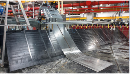
The 2D and 3D tests were conducted under identical boundary conditions to investigate the effect of the water body geometry on landslide-tsunamis. Figure 1 shows the set-up in the wave basin. Figure 2 shows a definition sketch of the measurement systems and parameters and the corresponding numerical values are included in Table 1. The slide made of PVC slid down on the PVC front of a ramp and the ramp face was inclined at α = 45°. A stainless steel guide in the centre of the ramp surface (Figure 1) matched a groove in the slide bottom to ensure that the slide remained in the channel centre during tsunami generation. A circular-shaped transition at the ramp toe was made of a stainless steel sheet bent to an eighth of a circle of radius 0.60 m and the facility bottom in the impact zone was covered with a stainless steel plate (see Figure 1 and attached file “Transition_geometry.stl”).

Figure 2. Side view of landslide-tsunami set-up and measurement system; the grey box shows the slide properties and force sensor locations in mm; the remaining dimensions are in m.

Table 1. Relevant parameters of 2D and 3D experiment with ρw as the water density; note that the wave profiles at all r/h and γ combinations were measured except for the combination r/h = 35.0 and γ = 90°.

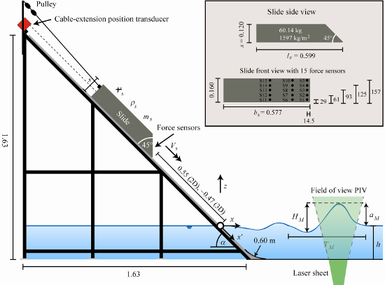
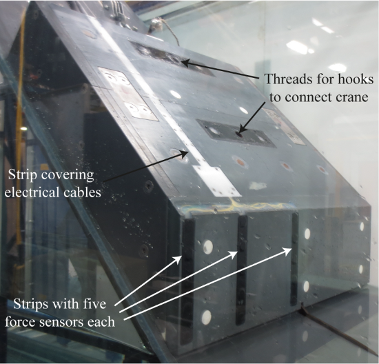
The slide surface is essentially flat, as shown in Figure 3, and the slide front angle is φ = 45°. The slide nose was trimmed by 6 mm and rounded. The slide length is ls = 0.599 m, the thickness s = 0.120 m, the mass ms = 60.14 kg, the volume Vs = 0.038 m3 and the density ρg = 1.597 kg/m3. The slide length is long enough to create a gap between the slide and the transition such that the slide is temporarily supported only at two contact points when it passes over the transition. The slide width bs = 0.577 m is smaller than the channel width b = 0.600 m resulting in a gap of 11.5 mm on either side. The slide geometry is available from the file “Slide_geometry.stl”. The slide nose was at x’ = ‒ 0.55 m in the release position in 2D and the slide was only moving due to gravity.

Figure 3. Slide in 2D: slide front with 15 force sensors, white PVC strip to cover electrical cables and threads for the hooks to connect the overhead crane.

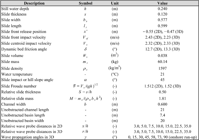
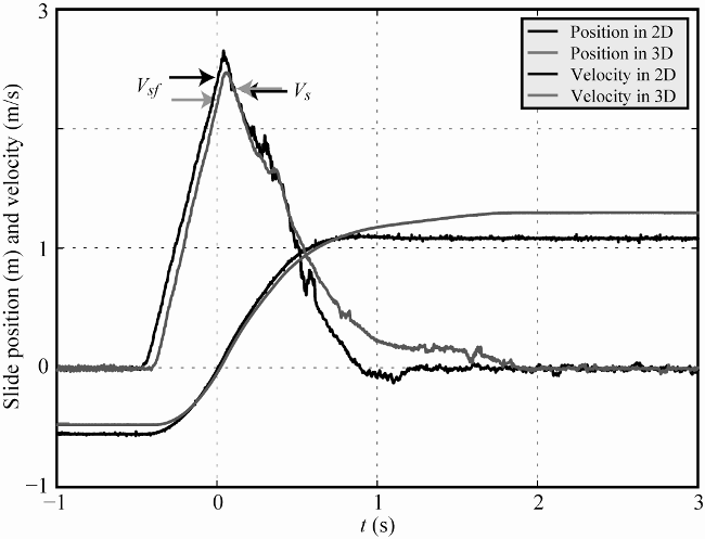
The position of the slide is shown in Figure 4 together with the slide velocity where the latter was directly derived from the slide position through numerical differentiation. The slide front impact velocities were 2.43 m/s (2D) and 2.23 m/s (3D) and the slide centroid impact velocities were Vs ≈ 2.32 m/s. The latter are practically identical as the tests were repeated until this was achieved; the slide front impact velocities deviate due to a small difference in the slide friction angles between 2D and 3D (Table 1) and wall effects in 2D. The dimensionless parameters are a slide Froude number F = Vs / (gh)1 / 2 ≈ 1.51 (with g as the gravitational acceleration), relative slide thickness S = s/h = 0.50 and relative slide mass M = ms / (ρw bh2) = 1.81 with ρw as the water density.

Figure 4. Slide positions and velocities versus time for 2D and 3D tests; the slide front reaches the still water surface (position = 0) at time t = 0, (data from “Position_and_velocity_2D.txt” and “Position_and_velocity_3D.txt”).

The coordinate origin is defined in the slide axis at the intersection of the still water surface and the hill slope ramp. The slide front reaches the water surface at time t = 0. All data in 2D and 3D were recorded along the slide axis (γ = 0) and for different slide propagation angles γ in 3D (Table 1). The measurement systems include a cable-extension position transducer measuring the entire slide kinematics in both 2D and 3D (Figure 4), 15 force sensors built in the slide front to measure the fluid forces during slide impact in 2D (Figure 6), PIV to measure the wave kinematics at various positions in 2D (Figure 8), resistance type wave gauges to measure the water surface elevation (Figure 7) both at 7 2D and at 48 3D locations (Table 1) and a video camera for optical observations (Figure 5, attached videos “2D.mp4” and “3D.mp4”).

Figure 5. Series of images of slide impact and tsunami generation in 3D with wave probes at 30° and 45°: (a) slide in release position, (b) slide impact crater and splash formation, (c) extending impact crater and splash hitting the first wave probes, (d) crater collapse and wave uprush in slide wake, (e) primary wave propagation on a semi-circle and (f) secondary wave generation by rundown of previous uprush; the time interval from (b) onwards is 0.2 s.

Figure 6. Pressure on slide front measured with S1, S3, S4 and S5 (Figure 2) in 2D. (data from “Pressures_2D.txt”).

Figure 7. Comparison of relative water surface elevations η/h versus relative time t(g/h)1/2 along the slide axis γ = 0° in both 2D (a-d) and 3D (e-h) at relative distance (a,e) x/h = r/h = 3.0, (b,f) 7.5, (c,g) 15.0 and (d,h) 35.0; note the increased scale on the ordinate in (f), (g) and (h) (data from “WGs_2D.txt” and “WGs_3D.txt”).

Figure 8. 2D wave kinematics measured with PIV over one wave period T at (a) x/h = 7.5 (T = 2.21 s), (b) 10.0 (T = 2.41 s) and (c) 15.0 (T = 2.82 s) relative to the linear shallow-water wave celerity (gh)1 / 2 = 1.53 m/s, (data from “Velocity_vectors_2D_7_5.txt”, “Velocity_vectors_2D_10_0.txt” and “Velocity_vectors_2D_15_0.txt”).

Boundary conditions

The slide release position in 3D was varied until the slide centroid impact velocity Vs was ±5% of the one previously measured in 2D. As a result, the actual release positions slightly differ in 2D and 3D. Note that the waves were measured with different ramp positions in the wave basin such that the primary wave is free of significant reflections. Significant reflections from the basin boundaries are expected later in the wave train. The 2D wave probe measurements are free from reflections for the entire presented time window.

Initial conditions

The overall geometry is defined under the “Geometry” section, Table 1 and Figure 2. The files defining the geometries of the slide and transition are attached (“Slide_geometry.stl”, “Transition_geometry.stl”) and they may be moved to the correct position with Paraview or a pre-processing interface and also integrated in the (XML) input file.

Fluid Properties

The fluid is incompressible and Newtonian.

Discretisation

A particle spacing of 10 mm may result in a good compromise between computational cost and achievable accuracy with respect to the water surface elevation. This resolution results in a total number of particles of about 1 million in 2D (involving all three spatial dimensions) with a domain length of 5 m and about 8 million in 3D with a domain size of 5 m × 6.5 m (Heller et al., 2016). However, a higher resolution is desirable for more exact results. One velocity vector in Figure 8 represents an interrogation window size of 15.5 mm × 15.5 mm. This is identical to the resolution in the attached files.

Results specification

A simulation may include the slide position and kinematics as shown in Figure 4. The position in Figure 4 follows x ' as long as the slide moves parallel to the ramp (until the slide front reaches the transition). For any subsequent times, the measured distance between slide rear and position sensor deviate from the x ' coordinate (Figure 2).

The force on the slide front may be compared with the measurements in Figure 6 to calibrate and validate fluid-structure interaction problems. In an engineering context, the water surface elevations at different positions are most relevant. This also includes the lateral onshore run-up in proximity of the impacting slide in 3D (Figure 1). This is often the area where the largest run-up height occurs, as landslide-tsunamis decay relatively fast in the offshore direction, e.g. with radial distance r−1 in 3D as an overall mean of the tests of Heller and Spinneken (2015). The water surface elevations along the slide axis are presented in Figure 7.

Wave kinematics (Figure 8) along with the surface elevation may support the calibration and validation of the coupling of SPH with a less computationally expensive code, e.g. based on the Boussinesq equations.

Results format

Slide kinematics: The slide position and velocity data in 2D shown in Figure 4 is available from the file “Position_and_velocity_2D.txt” of dimension 41,666 × 3 with column 1 = t (s) time at 8333 Hz, 2 = slide position (m) and 3 = slide velocity (m/s). The corresponding data in 3D is included in the file “Position_and_velocity_3D.txt” of dimension 9,920 × 3 with column 1 = t (s) time at 2024 Hz, 2 = slide position (m) and 3 = slide velocity (m/s).

Pressures: The pressures on the slide front are included in the file “Pressures_2D.txt” of dimensions 58,332 × 5 with column 1 = t (s) time at 8333 Hz, 2 = pressure at S1 (Pa), 3 = pressure at S3 (Pa), 4 = pressure at S4 (Pa) and 5 = pressure at S5 (Pa). Each sensor measured the pressure on a circular area of 12 mm in diameter.

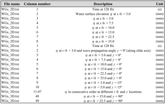
Water surface elevations: The water surface elevation data in 2D (Figure 7(a-d)) is included in the file “WGs_2D.txt” of dimension 1,280 × 8 and the water surface elevation data in 3D (Figure 7(e-h)) is presented in the file “WGs_3D.txt” of dimension 1,536 × 49. The data included in these two files are described in Table 2. Wave kinematics: The file “Velocity_vectors_2D_7_5.txt” includes the velocity vectors at resolution 15.5 mm × 15.5 mm as shown in Figure 8. The file dimension is 557 × 6 with column 1 = x-coordinate of velocity vectors over one wave period T (s), 2 = y-coordinate of velocity vectors over one T (s), 3 = x-component of velocity vectors (m/s), 4 = y-component of velocity vectors (m/s), 5 = t (s) of water surface elevation over one wave period and 6 = η (m) water surface elevation at x/h = 7.5. The two files “Velocity_vectors_2D_10_0.txt” and “Velocity_vectors_2D_15_0.txt” include the corresponding data in the identical order at x/h = 10.0 and x/h = 15.0, respectively.

Table 2. Description of data included in the water surface elevation files WGs_2D.txt and WGs_3D.txt; note that no measurements at the location r/h = 35.0 and γ = 90° were taken.

Benchmark results

The present benchmark test case is compared with numerical results in Heller et al. (2016) and the attached videos “2D.mp4” and “3D.mp4” give a general overview about the tests.

Figure 5 shows a picture series of tsunami generation in 3D with a description in the caption. The time interval from Figure 5(b) onwards is 0.2 s and these pictures may be used for a qualitative comparison with the numerical results.

Figure 6 shows the pressures measured on a circular area of 12 mm in diameter on the slide surface. They were measured with force sensors S1, S3, S4 and S5 in 2D (Figure 2). The pressure peak of 5.7 kPa is observed at S1 shortly after impact (t = 0). The pressure peaks of the remaining sensors S3, S4 and S5 are considerably smaller; for example, the pressure peak at S5, corresponding to the peak of 5.7 kPa at S1, is about 4.5 times smaller. Once the slide reaches the channel bottom, the pressure signals may be compared with the hydrostatic pressures based on still water conditions for each sensor (dashed lines in Figure 6). As expected, the pressures are larger than the hydrostatic pressure because the free water surface is moving and the sensors measure both the static and dynamic pressure components. The difference between the static pressure and the measured signal is in the order of 10% (Figure 6).

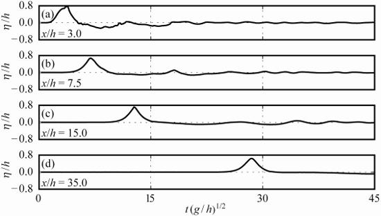
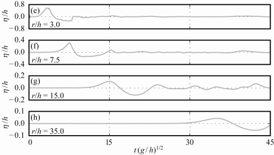
Figure 7 shows the relative water surface elevations η/h versus relative time t(g/h)1/2 for both 2D (a-d) and 3D (e-h) along the slide axis (γ = 0°) and for relative distances (a,e) x/h = r/h = 3.0, (b,f) 7.5, (c,g) 15.0 and (d,h) 35.0. Note that the scale on the ordinate in Figure 7(f), (g) and (h) is increased. Considerable differences between 2D and 3D are observed. The 2D wave is a solitary-like wave whereas the corresponding 3D wave is rather a Stokes-like wave. The wave profiles in 3D lie also lower relative to the still water surface and the tsunami in 3D is thus less non-linear than in 2D. The 2D wave amplitude close to the source (Figure 7(a)) is only 39% larger than in 3D (Figure 7(e)), whereas, further away at x/h = r/h = 35.0, the wave amplitude in 2D is a factor of 15.8 larger than in 3D due to lateral and radial energy spreading in 3D. This clearly demonstrates the importance of the water body geometry for tsunami features (Heller and Spinneken, 2015; Heller et al., 2016).

Figure 8 shows the velocity vectors over one wave period T at (a) x/h = 7.5 (with T = 2.21 s), (b) 10.0 (T = 2.41 s) and (c) 15.0 (T = 2.82 s). The reference vector corresponds to the linear shallow-water wave celerity (gh)1 / 2 = 1.53 m/s. The velocity vectors immediately below the highest crest elevation are about 90% of the reference velocity. As expected, a reverse water flow can be observed below the trough. Such wave kinematic plots give physical insight into the tsunami features and energy and may be useful to calibrate and validate the coupling of SPH with a less computational demanding code.

Suggestions

If you have something to add or if there is something else you think should be added, please write to valentin.heller@ nottingham.ac.uk.

References

Heller, V., and Spinneken, J. (2015). On the effect of the water body geometry on landslide-tsunamis - Physical insight from laboratory tests and 2D to 3D wave parameter transformation. Coastal Engineering, 104(10):113-134 (doi:10.1016/j.coastaleng.2015.06.006).

Heller, V., Bruggemann, M., Spinneken, J., and Rogers, B.D. (2016). Composite modelling of subaerial landslide-tsunamis in different water body geometries and novel insight into slide and wave kinematics. Coastal Engineering, 109(3):20-41 (doi:10.1016/j.coastaleng.2015.12.004).