(Download full test case data files here: SPHERIC_TestCase15.zip)

Introduction

Iceberg calving is the sudden release and breaking away of an ice mass from an iceberg, a glacier or an ice shelf. When icebergs calve into a water body, waves of tens of meters in height may be generated. Examples of such iceberg-tsunamis in Greenland include a 45 to 50 m amplitude wave observed at the Eqip Sermia glacier in 2014 and an event in 2018 where inhabitants of Innaarsuit had to be evacuated due to potential iceberg-tsunamis from icebergs detaching from a floating iceberg. A number of recent studies highlighted the hazards of such tsunamis, endangering the shipping industries, tourists and coastal communities.

Icebergs calve into a water body through different calving mechanisms (Benn et al., 2007). Heller et al. (2019; 2020) conducted laboratory experiments in a 50 m x 50 m large wave basin (Figure 1) to investigate the five idealized mechanisms A: capsizing, B: gravity-dominated fall, C: buoyancy-dominated fall, D: gravity-dominated overturning and E: buoyancy-dominated overturning. Gravity-dominated icebergs essentially fall into the water body whereas buoyancy-dominated icebergs essentially rise to the water surface.

Fig. 1 The 50 m x 50 m wave basin used for the experiments at Deltares, Delft.

This benchmark test case provides detailed laboratory data to calibrate and validate Smoothed Particle Hydrodynamics (SPH), and potentially other numerical methods such as the Immersed Boundary Method (Chen et al., 2020). In order to distinguish this test case from the subaerial landslide-tsunami cases provided in benchmark test cases 7 and 11, a capsizing and an overturning (gravity-dominated) test from the large-scale measurement campaign of Heller et al. (2019; 2020) were selected. The added challenge of these cases, compared to landslide-tsunamis, is to simulate both combined translational and rotational or pure rotational motion of icebergs, rather than solely a translation. Further, the generated deep-water waves are highly dispersive and quite small in the capsizing case.

The herein presented results include image series, the kinematics of the calving icebergs recorded by a motion sensor and wave profiles measured by 33 (capsizing) and 35 (overturning) resistance type wave probes located 2 to 35 m from the iceberg calving locations in different directions.

Flow phenomena

Fluid-structure interaction; Iceberg-tsunami generation and propagation; Violent three-phase flow; Turbulence; 3D rigid mass impact.

Geometry

The large-scale iceberg-tsunami tests were conducted in a 50 m x 50 m large wave basin, with an effective size (excluding wavemakers, absorbing beaches, etc.) of 40.3 m x 33.9 m (Figure 2). The water depth h was 1.0 m and the basin bottom was horizontal for both tests. Two square blocks made of polypropylene homopolymer and a density ρs ≈ 920 kg/m3, which is close to the density of ice, were used to model the icebergs. The dimensions of these two blocks are 0.800 m x 0.500 m x 0.500 m (block 1) and 0.800 m x 0.500 m x 0.250 m (block 2), respectively (Table 1). A purpose-built steel plate (Figure 3) was used to support the blocks before release.

Cylindrical coordinate systems (r, z, γ) were adopted in these tests with the coordinate origins shown in Figure 2. The origins are located for both calving mechanisms in vertical direction z on the still water surface with the z axes pointing upwards. In the horizontal plane the origin is located at the block centre for the capsizing case (Figure 2a) and at the front of the steel plate in the centre of the block in cross-shore direction for the overturning mechanism (Figure 2b). The wave propagation angle γ (angular angle) is defined positive in clockwise direction.

Two different triggering methods to release the blocks were used. Block 2 used in the capsizing case was hold in position with a wooden rod guided through the centre of the block (Figure 3a). The total mass of the block and rod combined was ms = 92.43 kg. This rod was hold in position on both sides with steel profiles rigidly connected to a steel plate lying flat on the basin bottom (Figure 3a). The steel profiles allowed the rod to heave and rotate (pitch) in the plane (r, z, γ = 0°). The rotation of the block was initiated by simply letting it go by hand. The block length was l = 0.800 m, the width b = 0.500 m and the thickness s = 0.250 m (Figures 2a and 3a, Table 1). Since the block was released at its equilibrium position in water, the release height (defined as the level of the block bottom above the still water surface) was −0.739 m.

For the gravity-dominated overturning case, block 1 rotated around a fixed axis defined with a steel rod of 30 mm diameter. This rod was fed through two ball bearings fixed to the block bottom surface (Figure 3b). This ensured that the block performed a pure rotation. The dimensions of the block in the overturning case were l = 0.800 m, b = 0.500 m and s = 0.500 m (Figures 2b and 3b, Table 1) and the mass ms = 187.11 kg. The release height was −0.300 m.

A 9 degrees of freedom motion sensor was fixed on the top face of the block (Figure 3) to record the block motion with a sampling frequency of 74Hz. The iceberg-tsunami features were measured with 33 (capsizing) and 35 (gravity-dominated overturning) resistance-type wave probes at a sampling frequency of 100Hz. Because the wave fields were symmetric, these wave probes were only placed in a semi-circle in the capsizing case and a quarter circle in the overturning case. Two cameras were used for general observations. Details about the locations of the waves probes and cameras are shown in Table 2. Two videos taken with one of the cameras are also attached in the folder of this benchmark test case. Based on two repetitions of the capsizing case and repetitions of some other calving scenarios not included herein, the measurement errors in Table 3 were estimated.

Fig. 2 Plan view of the (a) capsizing and (b) gravity-dominated overturning case. Some of the wave probes are numbered, with full details given in Table 2 (adapted from Heller, 2019).

Fig. 3 Sketches illustrating the two iceberg calving mechanisms: (a) capsizing and (b) gravity-dominated overturning case (adapted from Heller, 2019).

Table 1. Block dimensions and experimental parameters in the capsizing and gravity-dominated overturning cases. Note that the block densities changed slightly depending on the attachments (rod, clamp screws and bearings).

Table 2. Name and locations of wave probes and cameras.

Table 3. Measurement errors in the capsizing and overturning cases (adapted from Heller et al., 2019).

Boundary conditions

The block surfaces can all be modelled as no-slip solid boundary conditions. The fluid velocity on the solid surfaces (basin bottom and calving blocks) correspond to the velocity of the solid body. Note that only a part of the wave basin may be modelled for the tsunami generation. The results as input for a wave propagation model should then not be affected by reflections from the basin side walls.

Initial conditions

The water was still prior to releasing the blocks in both tests. In the capsizing test, the center of the block 1 was released in the center of the wave basin in the γ = 0° direction and 10.0 m from the basin side wall in the γ = 90° direction. In the gravity-dominated overturning case, block 2 was placed 10.9 m from the basin side wall in the γ = 90° direction. It is recommended to apply a small force in the order of 1 N to initiate block rotation in the same direction as in the laboratory tests. The masses and dimensions of the blocks can be found in the “Geometry” section and Table 1.

Discretisation

Experimental data are provided only.

Results specification

The result files contain the time history of the velocity and position of the tracking points (motion data), and the water surface elevations at the locations (wave probe data) shown in Table 2. Note that the motion sensor was located in a black enclosure fixed on the top surface of the blocks, the thickness of the enclosure base (3 mm) was also considered in the position. The tracking points are shown in Figure 3 (marked as yellow points), and at t = 0.0 s the tracking points were located at r = 0 m, z = 0.064 m, γ = 0° in the capsizing case and r = 0.25 m, z = 0.503 m, γ = 0° in the gravity-dominated overturning case, respectively. Attached are the processed tracking point velocity and position data files. Details on how to infer the trajectories of the tracking points using the motion sensor can be found in Chen et al. (2020).

Low-pass filters with cut-off frequencies between 3 and 11Hz were applied to remove noise in the wave probe data (Heller et al., 2020). Data contaminated by reflection were set to 0 in the attached water surface elevation data files.

Results format

Block kinematics (“post_processed_t1c_motion_capsizing_block2_100cm_-73.9cm” and “post_processed_t24_motion_overturning_gravity_block1_100cm_-30cm”): the data format is text (.txt). The file in each calving mechanism includes the displacement of the blocks in the r- and z-direction (γ = 0°). The data files are organized as follows:

column 1: time (s) with t = 0 s denoting when the blocks start to move,

column 2: horizontal velocity of the tracking point Vr (m/s) in x-direction,

column 3: vertical velocity of the tracking point Vz (m/s) in r-direction,

column 4: horizontal location of the tracking point (m) sr in x-direction,

column 5: vertical location of the tracking point (m) sz in r-direction.

Water surface elevations (“post_processed_t1c_waves_capsizing_block2_100cm_-73.9cm” and “post_processed_t24_waves_overturning_gravity_block1_100cm_-30cm”): the file format is also .txt and the files contain:

column 1: time (s) with t = 0 s corresponding to when the blocks start to move,

column 2-34 (capsizing case) and 2-36 (gravity-dominated overturning case): water surface elevations at each wave probe.

Benchmark results

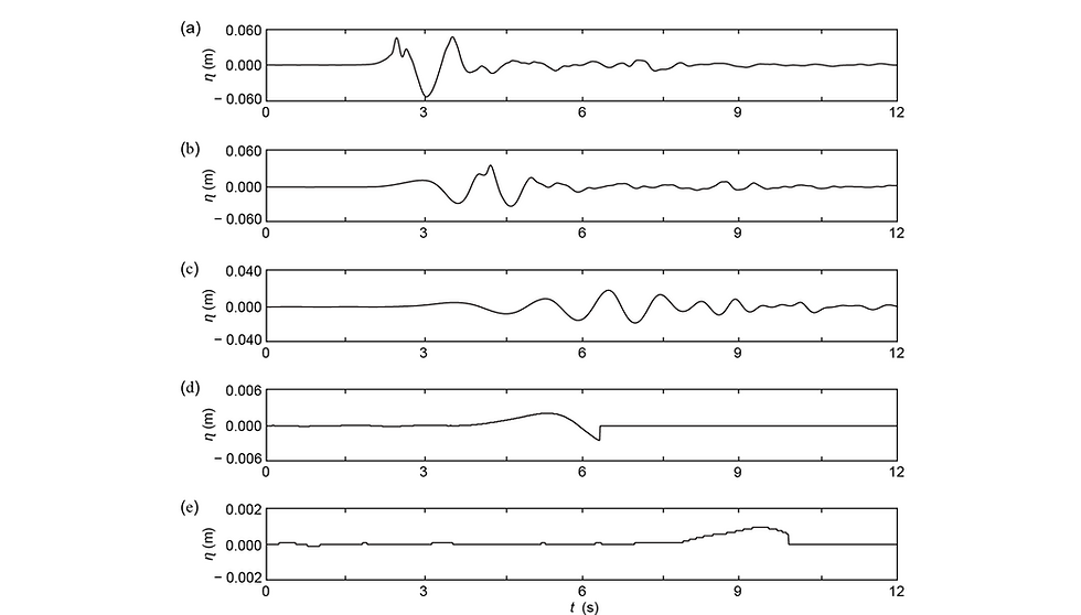
This benchmark test case includes one video for each calving mechanism to give a general overview. Photo series of the iceberg-tsunamis separated by 0.67 s are presented in Figures 4 and 5. Figure 6 shows the processed tracking point velocities and positions. z = 0.0 in the position figure corresponds to the water surface. Figures 7 and 8 show the generated tsunamis at wave probes A1, A10, A19 and A28 (capsizing case) and B1, B7, B13, B19 and B31 (gravity-dominated overturning case). The maximum possible resolution of the wave probe of 0.1 mm is reached in Figure 7d.

Figure 4 shows the evolution of the iceberg-tsunamis generated by the capsizing mechanism. The block started to overturn after release with the centre of rotation moving upwards. During the capsizing process some turbulence was generated, and the waves can be seen in the attached video. Figure 6a shows that the maximum velocity of the tracking point Vs,M = 0.21 m/s was reached at t = 2.6 s. The generated tsunamis can be seen in Figure 7 for γ = 0°, where the wave train reached wave probe A1 at t = 4.5 s and a maximum wave amplitude aM = 0.002 m and maximum wave height HM = 0.0036 m was observed. The wave decayed with distance and are significantly smaller at the remaining wave probes (Figure 7b,c,d).

Figure 5 shows the evolution of the iceberg-tsunamis generated in the gravity-dominated overturning test. The block rotated much faster than in the capsizing case and caused much more turbulence. A thin jet was generated by the rotating block (Figure 5d). The jet is expected to be well repeatable (estimated deviation of ±5% of the jet axis between repeats for a particular block position) as deviations would mainly propagate from the measurement error of the block velocity (Table 3). After the block fully submerged in water, a significant splash along γ = 0° was generated (Figure 5e). Figure 6c shows that the maximum velocity of the tracking point Vs,M = 1.92 m/s is an order of magnitude larger than for the capsizing case. The iceberg-tsunami reached its maximum wave amplitude aM = 0.047 m at wave probe B1 at t = 2.5 s and the first wave crest was affected by the splash (Figure 8a). Figure 8 shows the wave decay on the iceberg axis γ = 0°.

Fig. 4 Photo series of iceberg-tsunamis in the capsizing case at (a) t = 0.00 s, (b) t = 0.67 s, (c) t = 1.33 s, (d) t = 2.00 s, (e) t = 2.66 s and (f) t = 3.33 s.

Fig. 5 Photo series of iceberg-tsunamis in the gravity-dominated overturning case at (a) t = 0.00 s, (b) t = 0.67 s, (c) t = 1.33 s, (d) t = 2.00 s, (e) t = 2.66 s and (f) t = 3.33 s.

Fig. 6 Time history of (a,c) the tracking point motion and (b,d) positions in the (a,b) capsizing and (c,d) gravity-dominated overturning case.

Fig. 7. Time histories of iceberg-tsunamis generated in the capsizing case at wave probe (a) A1 (r = 2 m, γ = 0°), (b) A10 (r = 3 m, γ = 0°), (c) A19 (r = 5 m, γ = 0°) and (d) A28 (r = 10 m, γ = 0°). The wave probe signal reached its resolution limit in (d).

Figure 8. Time histories of iceberg-tsunamis generated in the gravity-dominated overturning case at wave probe (a) B1 (r = 2 m, γ = 0°), (b) B7 (r = 3 m, γ = 0°), (c) B13 (r = 5 m, γ = 0°), (d) B19 (r = 10 m, γ = 0°) and (e) B31 (r = 22.5 m, γ = 0°).

References

• Benn, D.I., Warren, C.R. and Mottram, R.H. (2007). Calving processes and the dynamics of calving glaciers. Earth-Science Reviews 82(3-4), 143-179.

• Chen, F., Heller, V. and Briganti, R. (2020). Numerical modelling of tsunamis generated by iceberg calving validated with large-scale laboratory experiments. Advances in Water Resources, 103647.

• Heller, V. (2019). Tsunamis due to ice masses: different calving mechanisms and linkage to landslide-tsunamis. Data storage report of HYDRALAB+ test campaign, online under http://hydralab.eu/research--results/ta-projects/project/hydralab-plus/11/.

• Heller, V., Attili, T., Chen, F., Gabl, R. and Wolters, G. (2020). Large-scale investigation into iceberg-tsunamis generated by various iceberg calving mechanisms. Coastal Engineering, 103745.

• Heller, V., Chen, F., Brühl, M., Gabl, R., Chen, X., Wolters, G. and Fuchs, H. (2019). Large-scale experiments into the tsunamigenic potential of different iceberg calving mechanisms. Scientific Reports 9, 861.

Acknowledgements

The large-scale laboratory tests were supported by the European Community's Horizon2020 Research and Innovation Programme through the grant to HYDRALAB+, Contract no. 654110.