Introduction

The present benchmark provides an approximate analytical solution of the Navier-Stokes equations for weakly-compressible fluids [1]. Such a solution resembles the classic Taylor-Green vortex [2] which, conversely, is valid for incompressible fluids.

Accordingly, the proposed solution is expected to be suitable for Weakly-Compressible SPH solvers in place of the classic Taylor-Green vortex. In particular, it is expected to drastically reduce the spurious acoustic noise that occurs as a consequence of the initialization through analytical solutions of incompressible flows.

Flow phenomena

• laminar viscous flow

• bi-periodic solution

• weakly-compressible fluid

Geometry

The geometry is a square with periodic boundary conditions (namely, a Torus). Specifically, the domain is D = [0, L*]² where L* denotes the length of the square side.

Boundary conditions

Periodic boundary conditions are assigned along the square sides.

Initial conditions

The initial conditions are obtained by computing the analytical solution at the time t=0. The latter is expressed in dimensionless variables through the following scaling (here the starred symbols are dimensional):

u* = U₀* u,      x* = L* x,      t* = T₀* t = L*/U₀* t,      p*=ρ₀* (U₀*)² p

where U₀*, L* and ρ₀* are respectively the reference velocity, the length of the square side and the reference density. The pressure and the density fields are related through a linear state equation that, in dimensionless variables, reads:

p = (ρ - 1)/ε        where       ε = (U₀*/c₀*)² = Ma²

Here c₀* is the sound velocity and Ma is the Mach number (Ma << 1 is assumed). The analytical solution is obtained through a perturbation expansion in terms of the parameter ε. In particular, the solutions for the density and the velocity field u = (u,v) are given by:

and the expansion of the pressure field is computed through the linear state equation, leading to ρ₁ = p₀ and ρ₂ = p₁ (where p₀ and p₁ are the zeroth- and first-order pressure solutions). Assuming the domain to be D = [0, 1]², the various contributions read:

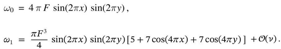
where F = exp (-8 π² 𝜈 t) and 𝜈 is dimensionless viscosity (namely the inverse of the Reynolds number Re = U₀* L* /𝜈*). The solutions for the vorticity field are:

Discretization

The initial discretization may be a uniform Cartesian lattice or, for SPH solvers, any regular particle distribution.

Results specification

Comparisons with the analytic solutions described in “Initial conditions”. For example:

·     time decay of the average kinetic energy per unit of mass for different Reynolds numbers.

·     convergence analysis on the average kinetic energy per unit of mass and/or on the pressure field at a fixed position for a chosen Reynolds number

·     contour maps of the velocity, pressure and vorticity fields

The figure below shows the contour plots of the various terms in the solutions of the pressure and vorticity fields:

Results format

Results are in the form of analytic expressions (see the section ”Initial conditions”).

Benchmark results

The analytical solution is particularly suited to test an SPH code for inviscid fluids. In this case, in fact, the acoustic noise generated by an inconsistent initialization is persistent in time and can jeopardize the simulation.

The Figure below shows the relative error of the pressure field measured at the center of the numerical domain when the simulation is initialized through the classic Taylor Green vortex (blue lines) or through the proposed weakly-compressible solution (red lines) for different Mach  numbers.

Download

You can download the full test case below:

References

• Antuono M. & Marrone S., “Weakly Compressible Approximation of the Taylor-Green Vortex Solution”, Studies in Applied Mathematics, 2024; 0:e12792, https://doi.org/10.1111/sapm.12792

• Taylor, G. I. (1923) LXXV. On the decay of vortices in a viscous fluid. Phil. Mag. 46, 671–674.